Warning: The theory hereby presented is not crystal clear. If you want, you can just look at the images...

Downloading: Click to download logconv-1.2.tar.gz. A copy of this documentation is provided with the source.

In this release: RGB support! Tooltips!

Compiling: After unpacking the source, just type configure and make install. logconv doesn't require any particular C function, so I suppose that all compilers will do the job. Of course, you will need the latest version of The GIMP and GTK+.

The Laplacian-of-Gaussian filter

The logconv filter for The GIMP implements an algorithm for edge detection developed in 1989 by Sotak and Boyer (read the article in Computer Vision, Graphics, and Image Processing 48, pgg. 147-189).

The Laplacian-of-Gaussian (LoG) operator has been suggested by Marr and Hildreth whilst studying the human visual system.
I will not explain you all the mathematics behind the development of this interesting filter (which you can read in the article cited above).
I will instead present you a few example of the use of this new operator and introduce you to the correct use of the parameters required by the filter.

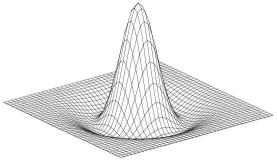
First of all, a perspective plot of the LoG operator.

Fascinating...

Then, the dialog of the LoG filter which you can find in The GIMP under Filter/Edge Detect/LoG

Cryptic...

Let's be serious. First of all, this implementation of the LoG works with rgb and grayscale images.
Now, let's look at the dialog window.
The Allowable PA is the percentage of allowable aliasing energy.
Technically speaking, it the amount of aliasing which can be tolerated. In practice, a bigger PA will produce small localization error of the edges. I hope to give you a more practical explanation soon...

Then, you have to choose between three different LoG implementations:

1. Standard LoG: The LoG convolution followed by a zero crossing of the resulting image
2. LoG with Roberts: The Standard LoG with a Roberts gradient.
3. LoG with Sobel: The Standard LoG with a Sobel gradient.

Finally, you must specify a standard deviation to apply to the LoG filter. In practice, the larger it is, the few details you'll get.
You can play with it but, in most cases, the suggested value of 2.0 will work quite well.

Now, a few examples...

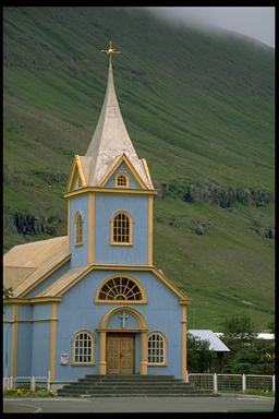This is a church in Seydisfjordur, Iceland.

Now we apply a standard LoG filter with PA=0.00001 and standard deviation of 2.0
Look at how well the church's contours are outlined. But you also get a lot of edges in the background, caused by small differences in the gray levels.
Notice that all contours are closed, an interesting property of the LoG filter.

Undo this filter and apply a LoG filter with Sobel gradient convolution, same parameters as before, PC1=25, PC2=60.
The image is now cleaner than before, but we have also lost details about the church.

Undo again. Apply now a standard LoG filter with PA=0.00001 and standard deviation of 4.0
Now the church is roughly outlined.

I think you'll make an artistic use of this filter.

_{Disclaimer: All photos from Corel Professional Photos CDs.}

_{Thanks: Many thanks to professor Boyer for providing me his articles.}